Research Notes: Differentiable Rendering

This post discusses the basics of differentiable rendering and is primarily a reading note from the SIGGRAPH 2020 Course.

This note comes from the course Physics-based differentiable rendering: from theory to implementation. The notes mainly focus on the theoretical derivations, as I’m not currently working on differentiable rendering, so the parts related to the rendering equation can be revisited later.

For more on automatic differentiation in rendering, you can also refer to Yzu-Mao Li's paper Systematically Differentiating Parametric Discontinuities published in SIGGRAPH 2021. The author implemented a Python DSL for autodiff why does everyone love Python so much, which might be helpful for autodiff in Luisa IR.

What is Differentiable Rendering?

Given all parameters \(\mathbb\pi\), rendering produces an image \(I(\mathbf\pi)\), and the loss function with respect to the ground truth image is \(L\). The goal of differentiable rendering is to compute \(\nabla_{\mathbf\pi}L(I(\mathbf\pi))\), enabling gradient-based optimization of rendering results for inverse rendering.

For any parameter \(\pi\) in \(\mathbf{\pi}\), we have: $$ \frac{\partial}{\partial\pi}L(I(\mathbf\pi)) = \sum_i\frac{\partial L}{\partial I_i(\mathbf{\pi})}\frac{\partial I_i(\mathbf{\pi})}{\partial\pi} $$ The first term is straightforward. For example, for the basic MSE Loss: $$ L = \left(I(\mathbf\pi) - \hat I(\mathbf\pi)\right)^2 $$

$$ \frac{\partial L}{\partial I(\mathbf{\pi})} = 2\left(I(\mathbf\pi) - \hat I(\mathbf\pi)\right) $$

The challenge lies in computing the latter term, \(\frac{\partial I_i(\mathbf{\pi})}{\partial\pi}\).

Can Rendering Be Made Differentiable "Painlessly"?

Rendering is essentially an integration problem. Take a simple anti-aliasing example: if each pixel is sampled at only one point, the result will have many jagged edges (high-frequency noise). One solution is to apply a low-pass filter, i.e., compute the integral over a region around the sampling center for each pixel: $$ I_i(\mathbf\pi) = \iint k(x,y)m(x_i+x, y_i+y; \mathbf\pi)\text{d}x\text{d}y = \iint f(x, y; \mathbf\pi)\text{d}x\text{d}y $$ where \(k\) is the convolution kernel, \(m\) is the continuous image space, and \(I\) is the discrete image. In practice, renderers typically use the following method (familiar as "Multisample Anti-Aliasing, MSAA") to numerically approximate this integral: $$ \iint f(x, y; \mathbf\pi)\text{d}x\text{d}y \approx \frac{1}{N}\sum_{j=1}^N f(x_j, y_j; \pi) $$ This numerical integration solves the computation of the integral but does not solve the differentiation of the integral: $$ \frac{\partial}{\partial \pi_v}\iint f(x, y; \mathbf\pi)\text{d}x\text{d}y \not\approx \frac{1}{N}\sum_{j=1}^N \frac{\partial}{\partial \pi_v}f(x_j, y_j; \mathbf\pi) = 0 $$

Why is the derivative of discrete sampling always 0?

The value of \(f(x_j, y_j; \mathbf\pi)\) is "the color of the object hit at this point." If the triangle hit doesn’t change when \(\pi_v\) changes, the gradient is necessarily 0; if it crosses a boundary, the gradient is theoretically infinite—but the probability of discrete sampling hitting the boundary is 0, so this term can be ignored.

Since differentiation is essentially about local changes, discrete sampling is insensitive to such changes, making direct differentiation of numerical integration infeasible. Consider a simpler example: $$ \frac{\partial}{\partial p}\int_0^1(x < p\ ?\ 1:0) \text{d}x $$ Discrete sampling will always yield 0, while the actual result is 1 (since the integral is simply \(p\)).

How to Differentiate This Integral?

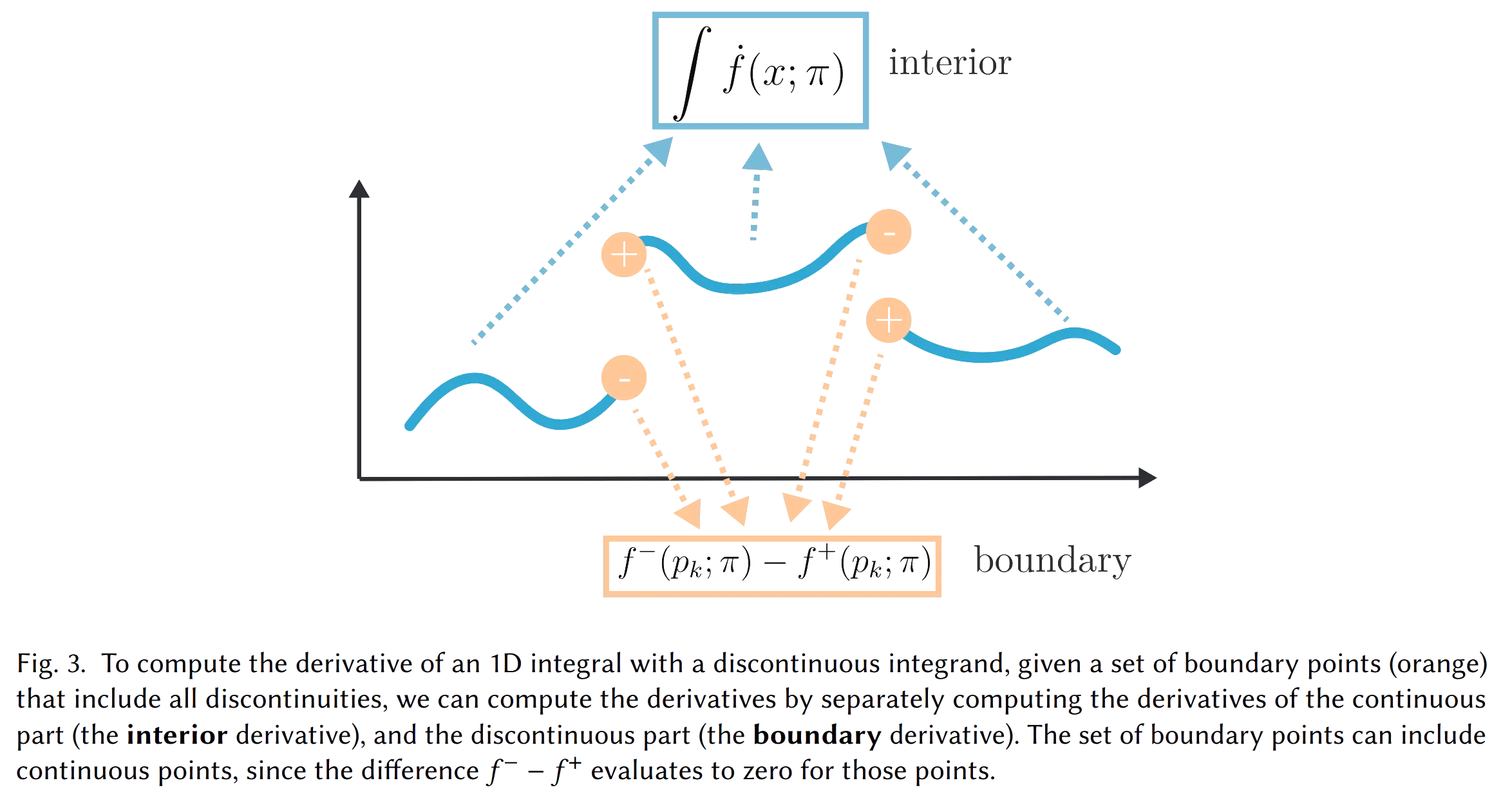
To compute the derivative of the integral of a discrete univariate function, first list all its discontinuities, then compute the derivatives of the continuous parts and the discontinuities separately.

For example, for the above integral: $$ \frac{\partial}{\partial p}\int_0^1(x < p\ ?\ 1:0) \text{d}x = \frac{\partial}{\partial p}\int_0^p 1\text{d}x + \frac{\partial}{\partial p}\int_p^1 0\text{d}x $$ Then compute each part separately. Generally: $$ \frac{\partial}{\partial\pi}\int_{a(\pi)}^{b(\pi)}f(x;\mathbf\pi)\text{d}x=\int_{a(\pi)}^{b(\pi)}\frac{\partial}{\partial\pi}f(x;\mathbf\pi)\text{d}x + \left[\frac{\partial b(\pi)}{\partial\pi}f(b(\pi); \mathbf\pi) - \frac{\partial a(\pi)}{\partial\pi}f(a(\pi); \mathbf\pi)\right] $$ The first term is the internal contribution, and the second term is the boundary compensation.

Extending to Higher Dimensions...

Let \(f\) be a function defined on an \(n\)-dimensional manifold \(\Omega(\pi)\), and \(\Gamma(\pi) \subset \Omega(\pi)\) be an \(n-1\)-dimensional manifold containing the external boundary \(\partial\Omega(\pi)\) and the boundaries between different regions within \(\Omega(\pi)\). Then, the derivative of the integral of \(f\) over \(\Omega(\pi)\) can be expressed as: $$ \frac{\partial}{\partial\pi}\left(\int_\Omega f\text{d}\Omega\right) = \int_\Omega\dot f \text{d}\Omega + \int_\Gamma\left\langle\mathbf{n}, \dot x\right\rangle \Delta f\text{d}\Gamma $$ where: $$ \dot f = \frac{\partial f}{\partial\pi} $$ $$ \dot x = \frac{\partial x}{\partial\pi} \ $$ $$ \Delta f(x) = \lim_{\epsilon\to0^-}f(x+\epsilon \mathbf n) - \lim_{\epsilon\to0^+}f(x+\epsilon \mathbf n) $$ Here, \(\dot x\) represents the direction of boundary movement as the parameter \(\pi\) changes. The two parts of the integral can be approximated numerically: $$ \int_\Omega\dot f \text{d}\Omega \approx \frac{1}{N_i}\sum_{j=1}^{N_i}\dot f(x_j) $$ $$ \int_\Gamma\left\langle\mathbf{n}, \dot x\right\rangle \Delta f\text{d}\Gamma \approx \frac{1}{N_b}\sum_{j=1}^{N_b}\left\langle\mathbf{n}, \dot x\right\rangle\Delta f(x_j) $$ Thus, we’ve addressed the theoretical problem of differentiable rendering...