Paper Note: Radiative Backpropagation

This article discusses Radiative Backpropagation for differentiable rendering.

Introduction

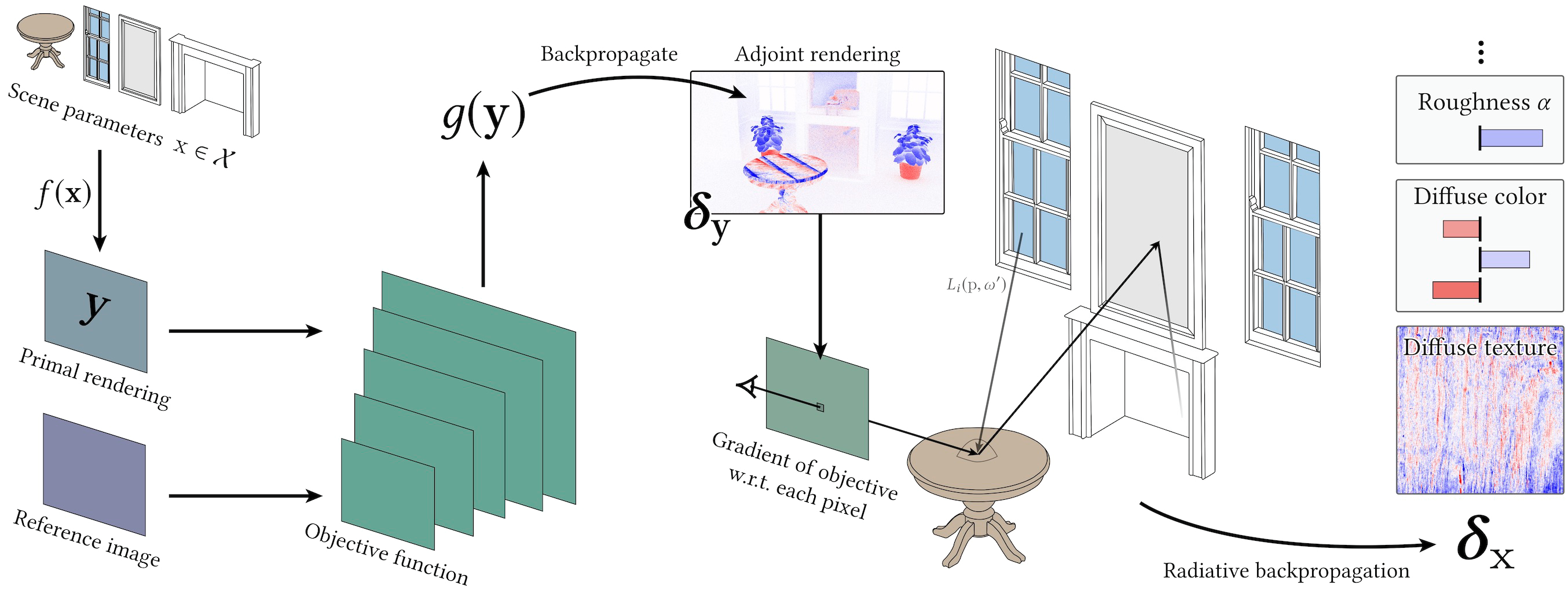
Formalize the scene parameters as \(\mathbf{x}\) and the rendering function as \(f\). The process of computing \(\mathbf{y} = f(\mathbf{x})\) is the forward rendering process.

Differentiable rendering aims to compute: $$ \mathbf{J}_f := \frac{\partial f(\mathbf{x})}{\mathbf x} $$ Since the spaces of \(\mathbf{x}\) and \(\mathbf{y}\) are high-dimensional, directly computing \(\mathbf{J}_f\) is infeasible. Therefore, existing methods are mainly divided into two categories:

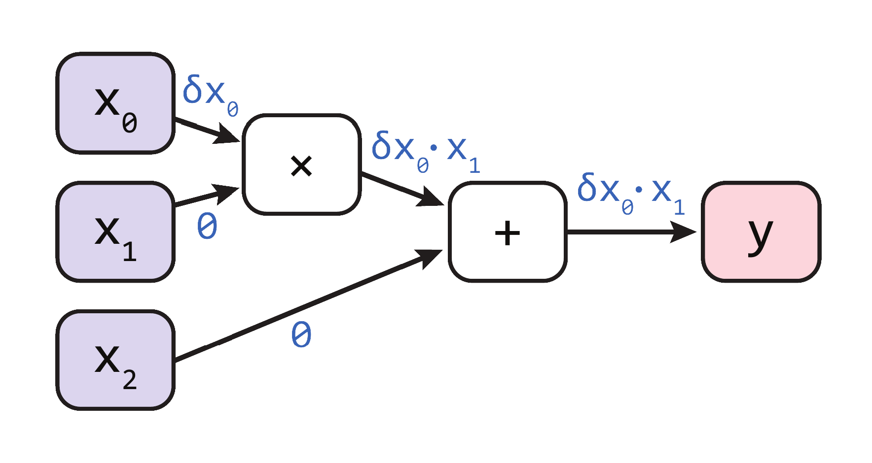
• Forward-mode methods: Compute the effect of a small perturbation \(\mathbf{\delta_x}\) on \(\mathbf{y}\) as \(\mathbf{\delta_y} = \mathbf{J}_f\mathbf{\delta_x}\).
• Reverse-mode methods: Compute the small perturbation \(\mathbf{\delta_x}\) in \(\mathbf{x}\) required to produce a change \(\mathbf{\delta_y}\) in \(\mathbf{y}\) as \(\mathbf{\delta_x} = \mathbf{J}_f^T\mathbf{\delta_y}\).

For example, to compute the gradient of \(y = x_0 \times x_1 + x_2\), the forward and reverse methods are illustrated below:

In reverse-mode methods, the most common approach is auto-differentiation based on tracing, where the computational graph is recorded during forward computation and then backpropagated. However, this method requires recording a large amount of information on the computational graph during forward computation, resulting in high memory consumption and slow computation.

Radiative Backpropagation provides a reverse-mode method with lower memory and time overhead. It does not require recording the computational graph during forward computation but instead precomputes certain elements and performs backpropagation after forward rendering.

Theory

Assumptions

The derivation makes the following assumptions:

• Volumetric effects are not considered.
• Gradients caused by silhouette boundaries are not considered.

Three Fundamental Equations of Rendering

Measurement Equation

Let each pixel in the image be \(I_1, I_2, \cdots, I_n\). The measurement value of the \(k\)-th pixel is the inner product of \(W_k\) and \(L_i\) in the space \(\mathcal{A} \times S^2\), i.e.: $$ I_k = \left\langle W_k, L_i\right\rangle = \int_{\mathcal{A}}\int_{S^2}W_k(\mathbf{p},\mathbf{\omega})L_i(\mathbf{p},\mathbf{\omega})\text{d}\mathbf{\omega}^{\perp}\text{d}\mathbf{p} $$ where \(W_k\) is the importance function of \(I_k\), \(L_i\) is the incident radiance, \(\mathcal{A}\) represents all points, and \(S^2\) represents the hemisphere.

Transport Equation

For unoccluded rays, the incident radiance equals the outgoing radiance at the exit point, i.e.: $$ L_i(\mathbf{p},\mathbf{\omega}) = L_o(\mathbf{r}(\mathbf{p},\mathbf{\omega}), -\mathbf{\omega}) $$ where \(\mathbf{r}(\mathbf{p},\mathbf{\omega})\) represents the nearest intersection point along the ray \((\mathbf{p},\mathbf{\omega})\), i.e., the exit point of this ray.

Note that the assumption of no occlusion plays a role here.

Scattering Equation

For a point, the relationship between its outgoing radiance and incident radiance can be expressed as: $$ L_o(\mathbf{p},\mathbf{\omega}) = L_e(\mathbf{p},\mathbf{\omega}) + \int_{S^2}L_i(\mathbf{p},\mathbf{\omega'})f_s(\mathbf{p},\mathbf{\omega},\mathbf{\omega'})\text{d}\mathbf{\omega'}^{\perp} $$ where \(L_e(\mathbf{p},\mathbf{\omega})\) is the emitted radiance, and \(f_s(\mathbf{p},\mathbf{\omega},\mathbf{\omega'})\) is the BSDF. This equation is commonly known as the "rendering equation."

Differential Forms of the Three Equations

For convenience, let the partial differential operator \(\frac{\partial}{\partial \mathbf{x}}\) be denoted as \(\partial_\mathbf{x}\).

Measurement Equation

$$ \partial_{\mathbf{x}}I_k = \int_{\mathcal{A}}\int_{S^2}W_k(\mathbf{p},\mathbf{\omega})\partial_\mathbf{x}L_i(\mathbf{p},\mathbf{\omega})\text{d}\mathbf{\omega}^{\perp}\text{d}\mathbf{p} $$

Note that there is no gradient of \(W_k\) here, as we assume no occlusion, so the importance remains unchanged.

Transport Equation

$$ \partial_\mathbf{x}L_i(\mathbf{p},\mathbf{\omega}) = \partial_\mathbf{x}L_o(\mathbf{r}(\mathbf{p},\mathbf{\omega}), -\mathbf{\omega}) $$

Scattering Equation

$$ \partial_\mathbf{x}L_o(\mathbf{p},\mathbf{\omega}) = \partial_\mathbf{x}L_{e}(\mathbf{p},\mathbf{\omega}) + \int_{S^2}[\partial_\mathbf{x}L_i(\mathbf{p},\mathbf{\omega'})f_s(\mathbf{p},\mathbf{\omega},\mathbf{\omega'}) + L_i(\mathbf{p},\mathbf{\omega'})\partial_\mathbf{x}f_s(\mathbf{p},\mathbf{\omega},\mathbf{\omega'})]\text{d}\mathbf{\omega'}^{\perp} $$

The right-hand side of the equation contains three terms with \(\partial_{\mathbf{x}}\):

• \(\partial_{\mathbf{x}}L_e(\mathbf{p},\mathbf{\omega})\)

  If the scene parameter \(\mathbf{x}\) is perturbed and the light source's brightness changes, it "emits" differential radiance.

• \(\partial_\mathbf{x}L_i(\mathbf{p},\mathbf{\omega'})f_s(\mathbf{p},\mathbf{\omega},\mathbf{\omega'})\)

  Differential radiance is "scattered" like regular radiance.

• \(L_i(\mathbf{p},\mathbf{\omega'})\partial_\mathbf{x}f_s(\mathbf{p},\mathbf{\omega},\mathbf{\omega'})\)

  If the scene parameter \(\mathbf{x}\) is perturbed and the material changes, this BSDF also "emits" differential radiance.

Optimizing Differential Computation

Given an optimization objective, let the loss function be \(g\) and the rendering function be \(f\). We need to compute: $$ \partial_{\mathbf{x}}g(f(\mathbf{x})) = \mathbf{J}_{g \circ f}(\mathbf{x}) = \mathbf{J}_g(f(\mathbf{x}))\mathbf{J}_f(\mathbf{x}) $$ We break this into two steps:

1. First, compute \(\mathbf{\delta_y} = \mathbf{J}^T_g(\mathbf{y})\). This can be done manually or via auto-differentiation.
2. Then, use radiative backpropagation to compute \(\mathbf{\delta_x} = \mathbf{J}^T_f\mathbf{\delta_y}\).

Computing \(\mathbf{J}^T_f\mathbf{\delta_y}\)

Express \(\mathbf{J}f\) as a column vector: $$ \mathbf{J}{f} = [\partial_{\mathbf{x}}I_0, \cdots, \partial_{\mathbf{x}}I_n] $$

Thus: $$ \mathbf{J}^T_f\mathbf{\delta_y} = \sum_{k=1}^n\mathbf{\delta}_{\mathbf{y},k}\partial_{\mathbf{x}}I_k = \int_{\mathcal{A}}\int_{S^2}\left[\sum_{k=1}^n\mathbf{\delta}_{\mathbf{y},k}W_k(\mathbf{p},\mathbf{\omega})\right]\partial_\mathbf{x}L_i(\mathbf{p},\mathbf{\omega})\text{d}\mathbf{\omega}^{\perp}\text{d}\mathbf{p} $$

Define the "emitted adjoint radiance": $$ A_e(\mathbf{p},\mathbf{\omega}) := \sum_{k=1}^n\mathbf{\delta}_{\mathbf{y},k}W_k(\mathbf{p},\mathbf{\omega}) $$ After computing \(\mathbf{\delta_y}\), \(A_e\) can be trivially computed.

Referencing the measurement equation, we can write: $$ \mathbf{J}^T_f\mathbf{\delta_y} = \langle A_e, \partial_{\mathbf{x}}L_i \rangle $$

Let: $$ \mathbf{Q}(\mathbf{p},\mathbf{\omega}) := \partial_{\mathbf{x}}L_e(\mathbf{p},\mathbf{\omega}) + \int_{S^2}L_i(\mathbf{p},\mathbf{\omega'})\partial_{\mathbf{x}}f_s(\mathbf{p},\mathbf{\omega},\mathbf{\omega'})\text{d}\mathbf{\omega'}^{\perp} $$

Additionally, define two operators: the scattering operator \(\mathcal{K}\) and the transport operator \(\mathcal{G}\) as: $$ (\mathcal{K}h)(\mathbf{p},\mathbf{\omega}) := \int_{S^2}h(\mathbf{p},\mathbf{\omega'})f_s(\mathbf{p},\mathbf{\omega},\mathbf{\omega'})\text{d}\mathbf{\omega'} $$ $$ (\mathcal{G}h)(\mathbf{p},\mathbf{\omega}) := h(\mathbf{r}(\mathbf{p},\mathbf{\omega}), -\mathbf{\omega}) $$

Based on these definitions, we obtain two equations: $$ \partial_{\mathbf{x}}L_i = \mathcal{G}\partial_{\mathbf{x}}L_o $$ $$ \partial_{\mathbf{x}}L_o = \mathcal{K}\partial_{\mathbf{x}}L_i + \mathbf{Q} $$

These correspond to the transport and scattering equations, respectively. According to a 1997 paper by Veach, we can directly derive some conclusions, such as: $$ \partial_{\mathbf{x}}L_o = \mathcal{KG}\partial_{\mathbf{x}}L_o + \mathbf Q = (I - \mathcal{KG})^{-1}\mathbf{Q} = \sum_{i=0}^{\infty}(\mathcal{KG})^i\mathbf Q $$

Let \(\mathcal S := (I - \mathcal{KG})^{-1}\). Then, \(\mathcal {G, K, GS}\) are all self-adjoint linear operators.

A linear operator \(\mathcal O\) is self-adjoint if \(\forall v_1, v_2\), \(\langle \mathcal Ov_1, v_2\rangle = \langle v_1,\mathcal{O}v_2\rangle\).

Therefore: $$ \mathbf{J}^T_f\mathbf{\delta_y} = \langle A_e, \partial_{\mathbf{x}}L_i \rangle = \langle A_e, \mathcal{GS}\mathbf{Q} \rangle = \langle \mathcal{GS}A_e, \mathbf{Q} \rangle $$

Applying the \(\mathcal{GS}\) operator to \(A_e\) does not change the result, essentially indicating that we can "start from the other side" to scatter and transport radiance, and the result remains the same. Since \(A_e\) is a scalar function and \(\mathbf Q\) is a vector function with the same dimension as \(\mathbf{x}\) (making it impossible to compute), applying the self-adjoint property makes it much easier to compute.

After obtaining \(A_e\), we define similar "incident adjoint radiance" and "outgoing adjoint radiance" \(A_i, A_o\) as: $$ A_i = \mathcal{G}A_o $$ $$ A_o = \mathcal{K}A_i + A_e $$

Thus, we have adjoint radiance \(A_e, A_o, A_i\) that satisfies the fundamental rendering equations, turning backpropagation into "another forward rendering."

Pseudocode

def grad(x):
    # Forward rendering
    y = f(x)
    # Compute the differential of y
    delta_y = J_g(y)
    # Use radiative backprop to compute the differential of x
    return radiative_backprop(x, delta_y)

def radiative_backprop(x, delta_y):
    delta_x = 0
    for _ in range(num_samples):
        # Importance sample a ray
        p, omega, weight = sensor.sample_ray()
        # Compute emitted adjoint radiance
        weight *= A_e(delta_y, p, omega) / num_samples
        # Propagate adjoint radiance in the scene
        delta_x += radiative_backprop_sample(x, p, omega, weight)
    return delta_x

def radiative_backprop_sample(x, p, omega, weight):
    # Find the intersection point
    p_prime = r(p, omega)
    # If this point has emitted radiance (light source), add its contribution to the differential
    delta_x = adjoint([[ L_e(p_prime, -omega) ]], weight)
    # Sample a ray from the BSDF
    omega_prime, bsdf_value, bsdf_pdf = sample(f_s(p_prime, -omega, ·))
    # If this BSDF contributes to the differential, add it
    delta_x += adjoint([[ f_s(p_prime, -omega, omega_prime) ]],
                       weight * L_i(p, omega_prime) / bsdf_pdf)
    
    # Recursive step
    return delta_x + radiative_backprop_sample(x, p_prime, omega_prime, 
                                               weight * bsdf_value / bsdf_pdf)

The adjoint([[ q(z) ]], delta) function propagates the gradient \(\mathbf{\delta}\) to \(q\) (by computing \(\mathbf{J}_q^T(\mathbf{x},\mathbf{z})\mathbf{\delta}\)) and returns the gradient with respect to \(\mathbf{x}\).

Optimization

Using Biased Gradient Estimation for Speedup

Change the definition of \(\mathbf{Q}\) from: $$ \mathbf{Q}(\mathbf{p},\mathbf{\omega}) := \partial_{\mathbf{x}}L_e(\mathbf{p},\mathbf{\omega}) + \int_{S^2}L_i(\mathbf{p},\mathbf{\omega'})\partial_{\mathbf{x}}f_s(\mathbf{p},\mathbf{\omega},\mathbf{\omega'})\text{d}\mathbf{\omega'}^{\perp} $$ to: $$ \mathbf{Q}_{\text{approx}}(\mathbf{p},\mathbf{\omega}) := \partial_{\mathbf{x}}L_e(\mathbf{p},\mathbf{\omega}) + \int_{S^2}\partial_{\mathbf{x}}f_s(\mathbf{p},\mathbf{\omega},\mathbf{\omega'})\text{d}\mathbf{\omega'}^{\perp} $$ i.e., directly remove the incident radiance (set it to 1). This avoids recursively computing incident radiance during radiative backprop.

Surprisingly, this not only speeds up computation but also improves convergence.

Reusing Intermediate Results for Speedup

The authors note that many intermediate results in radiative backpropagation are the same as in forward rendering (e.g., BSDF sampling results, MIS weights). Therefore, we can perform backpropagation and the next forward rendering together, sampling only once.

This essentially uses the gradient of \(\mathbf{y}\) from the previous iteration to propagate the gradient of \(\mathbf{x}\) in the current iteration, which is valid if the gradient changes smoothly.

The pseudocode for this optimization is:

def grad_optimized(x):
    y = f(x)
    while not converged:
        delta_y = J_g(y)
        # Radiative backprop also renders the next y
        y, delta_x = radiative_backprop(x, delta_y)
        # Propagate gradient ...