Paper Note: Spatiotemporal reservoir resampling for real-time ray tracing with dynamic direct lighting

August 6, 2023 ·

This article discusses the theoretical foundation and implementation of the ReSTIR algorithm.

Preface

The renowned ReSTIR sampler achieves highly efficient sampling using a very simple data structure.

The core idea is to use Weighted Reservoir Sampling (WRS) for Resampled Importance Sampling (RIS), and then leverage the properties of WRS to add low-overhead temporal and spatial sampling reuse.

Subsequently, the article analyzes the situations and reasons that lead to bias and provides an unbiased version of the algorithm.

Update as of Dec. 2024

This blog was written when I just finished the paper reading and did not have a very good understanding of the algorithm. It is quite superfluent by my today's view, and I may give it a rewrite in the future.

Problem Statement

The rendering equation is essentially an integral. For example, the radiance emitted from point $y$ in direction $\vec{\omega}$ is: $$ L(y,\omega) = \int_A \rho(y, \vec{yx}\leftrightarrow \vec{\omega}) \cdot L_e(x\to y)\cdot G(x\leftrightarrow y)V(x\leftrightarrow y)\text{d}A_x $$ where $\rho$ is the BRDF, $L_e$ is the outgoing radiance from the previous point $x$, $V$ is visibility, and $G$ is the geometric term (i.e., the cosine of the angle with the normal). Simplified, it can be written as: $$ L= \int_Af(x)\text{d}x, f(x) =\rho(x)L_e(x)G(x)V(x) $$ The rendering process involves discretely sampling and estimating this integral.

Importance Sampling (IS)

Starting from a PDF $p$ that approximates $f$, sample $N$ samples $x_1, x_2, \cdots, x_n$ with weights $p$: $$ \langle L \rangle^N_{\text{is}} = \frac{1}{N}\sum_{i=1}^N\frac{f(x_i)}{p(x_i)} $$ As long as $f$ is non-zero and $p$ is always positive, IS is unbiased; the closer $p$ is to $f$, the lower the variance.

The problem with IS is that although some components of $f$ (e.g., $L_e, \rho$) have known PDFs, it is difficult to find a PDF that closely approximates $f$ itself.

Multiple Importance Sampling (MIS)

MIS addresses the difficulty of fitting the integrand in IS by using different strategies and weighted combinations. It uses easily fitted weights like $L_e$ and $\rho$ and then mixes the sampling results with weights: $$ \langle L\rangle_{\text{mis}}^{M,N} = \sum_{s=1}^M\frac{1}{N_s}\sum_{i=1}^{N_s}w_s(x_i)\frac{f(x_i)}{p_s(x_i)} $$ where $M$ is the number of sampling strategies (i.e., the number of PDFs) and $N_s$ is the number of samples for each strategy. As long as the weights $w_s$ sum to 1 across strategies, MIS remains unbiased.

In practice, the weights are often set as the product of the number of samples and the probability density: $$ w_s(x) = \frac{N_sp_s(x)}{\sum_jN_jp_j(x)} $$

Resampled Importance Sampling (RIS)

Unlike MIS, RIS does not use linear weighted combinations to fit the integrand.

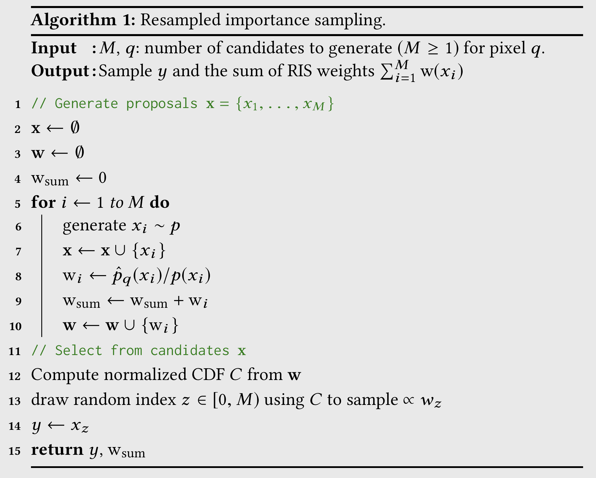
Assume the ideal distribution is $\hat p$ (e.g., $\hat p\propto\rho\cdot L_e\cdot G$). RIS starts with a potentially poor distribution $p$ (e.g., $p \propto L_e$) and samples $M$ samples $x_1, x_2, \cdots x_M$. Then, it resamples from these $M$ samples with weights $\text{w}$: $$ \text{w}(x) = \frac{\hat{p}(x)}{p(x)} $$ The resampled sample is named $y$, and the estimate is: $$ \langle L\rangle_{\text{ris}}^{1,M} = \frac{f(y)}{\hat p(y)}\cdot\left(\frac{1}{M}\sum_{j=1}^M\text{w}(x_j)\right) $$ Repeating this process $N$ times and averaging yields the RIS estimate: $$ \langle L\rangle_{\text{ris}}^{N,M} = \frac{1}{N}\sum_{i=1}^{N}\left(\frac{f(y_i)}{\hat p(y_i)}\cdot\left(\frac{1}{M}\sum_{j=1}^M\text{w}(x_{ij})\right)\right) $$ This form resembles IS, but since $y_i$ is not directly sampled from $\hat p$ but resampled from $p$, a compensation term involving $\text{w}$ is added to each $f(y_i)$ to ensure unbiasedness.

As $M \to \infty$, the distribution of $y$ approaches $\hat p$; however, for finite $M$, the quality of $p$ is also crucial for sampling effectiveness.

The pseudocode for a single RIS iteration is:

Weighted Reservoir Sampling (WRS)

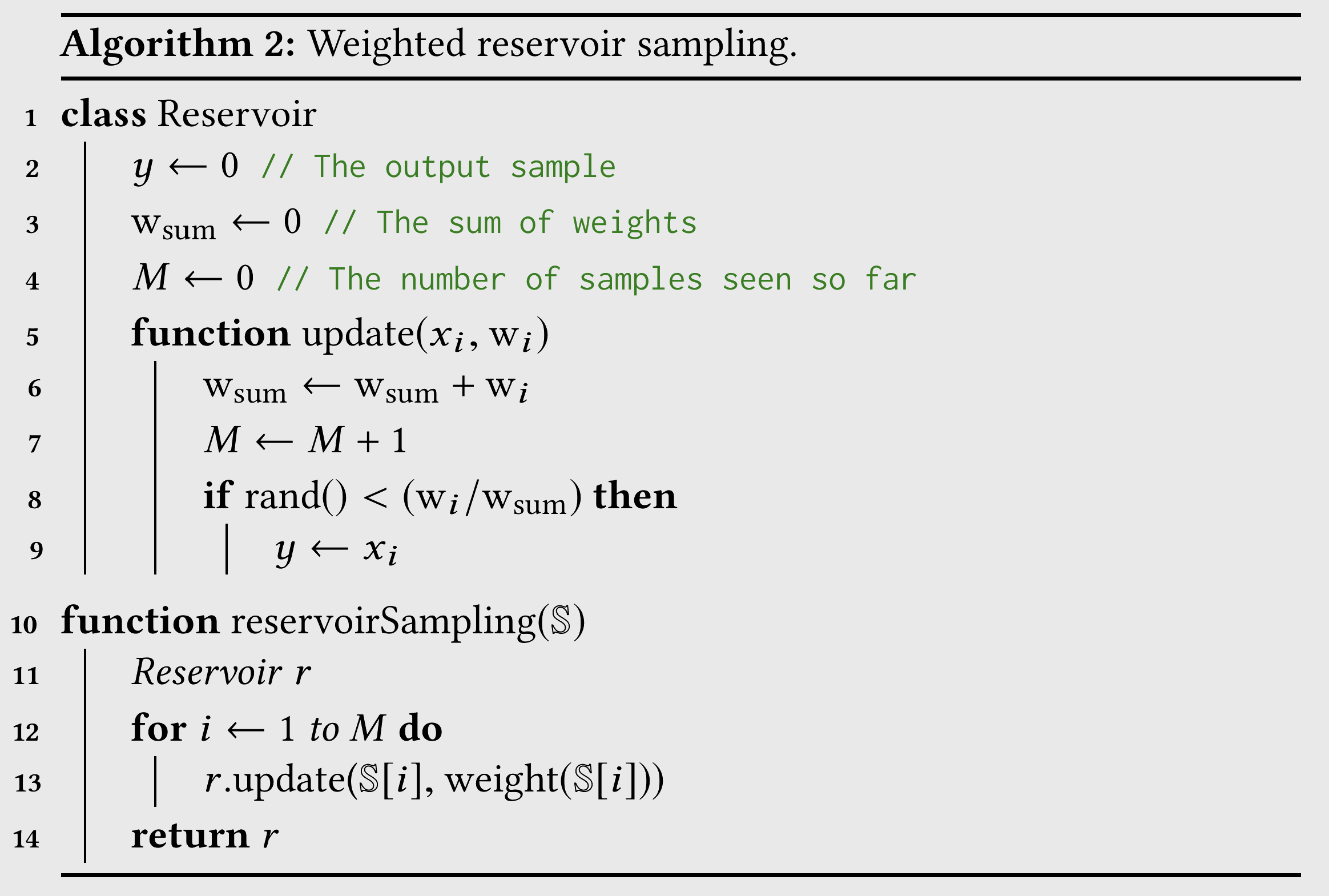
Given a stream of $M$ values, each with weight $w_i$, WRS selects $N$ samples in a single pass based on their weights ($M$ is unknown at the start and is updated incrementally).

Here, we simplify $N$ to 1, selecting only one sample.

The pseudocode for WRS is as follows, where a reservoir structure is defined, essentially dynamically maintaining the "currently selected sample." Each time a new value is obtained from the stream, it is randomly decided whether to replace the current sample:

Stream RIS (Combining WRS and RIS)

By optimizing the $M$ samples of RIS using WRS, the number of samples can be increased while reducing memory usage.

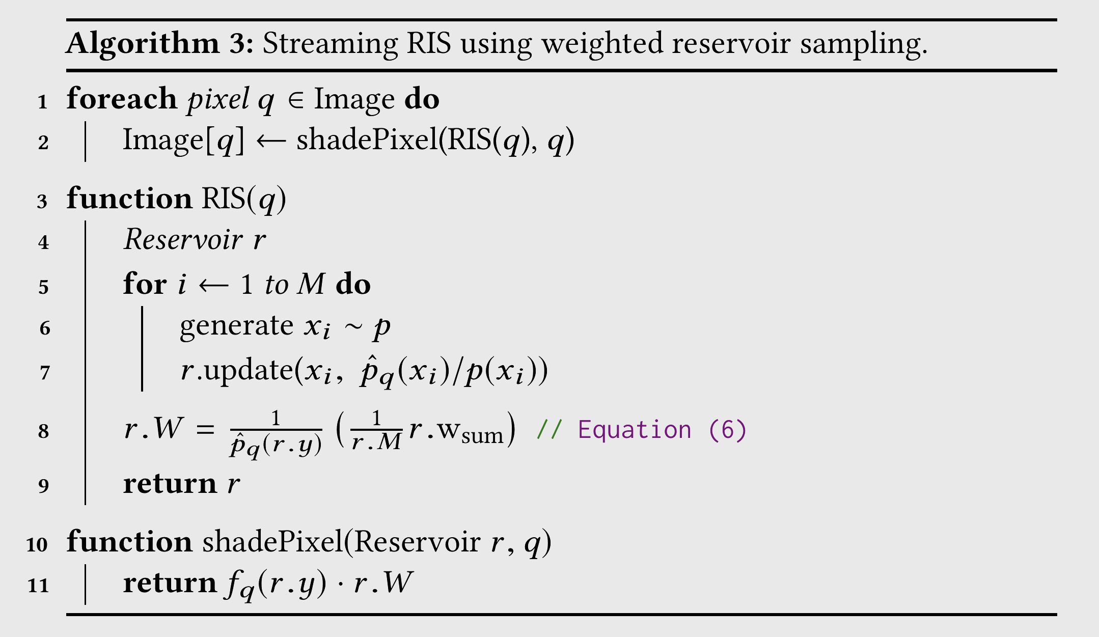
Using stream RIS alone for sampling, the pre-denoised results are already significantly better than LightBVH under the same computational power and time, and the time required for the same quality is shorter.

Note that a new field $W$ is introduced to the reservoir, which corresponds to the part of the RIS estimate: $$ \langle L\rangle_{\text{ris}}^{1,M} = \frac{f(y)}{\hat p(y)}\cdot\left(\frac{1}{M}\sum_{j=1}^M\text{w}(x_j)\right) $$ excluding $f(y)$.

Temporal and Spatial Reuse

Spatial Reuse

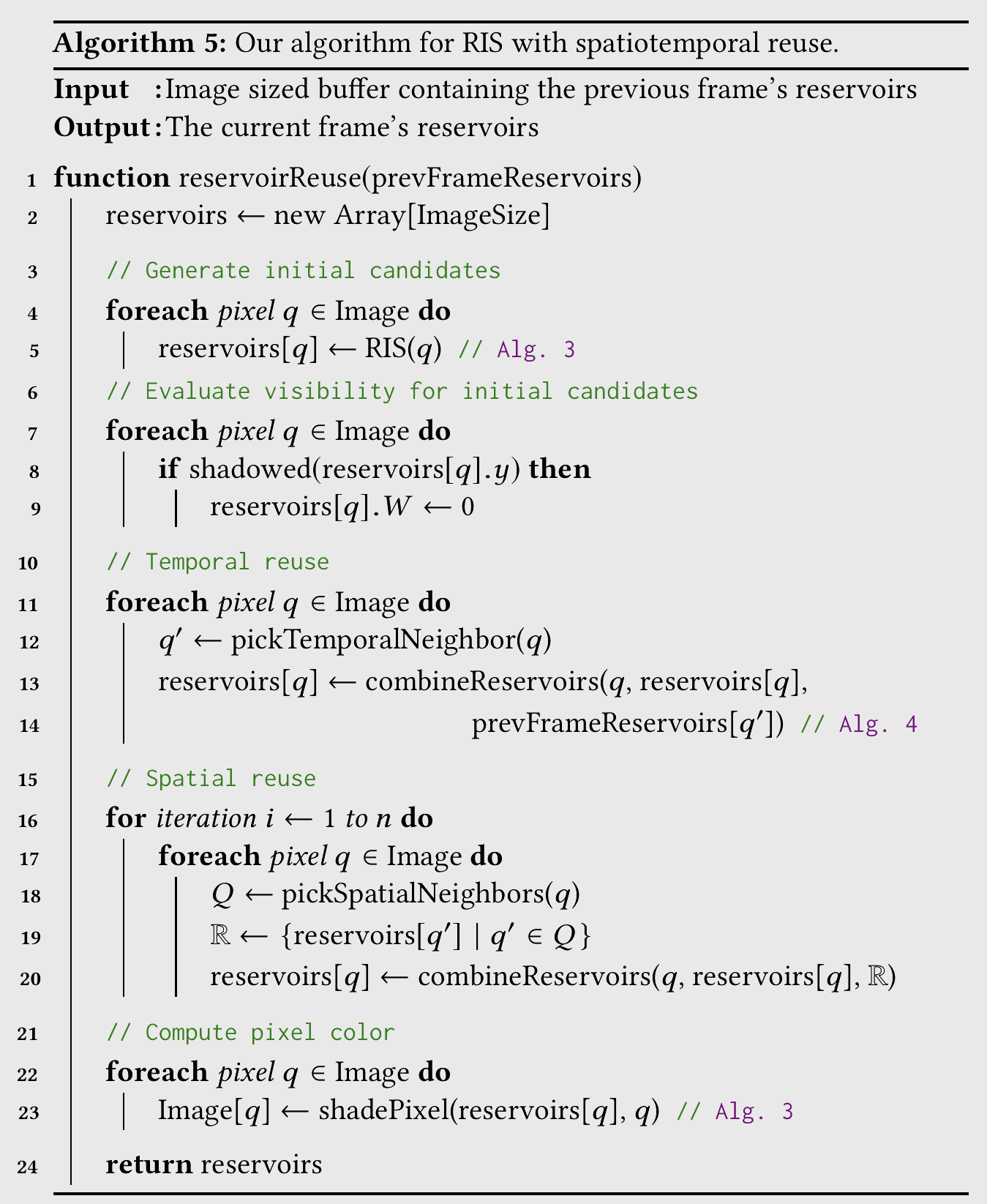
Ignoring the occlusion term $V$, we often assume that neighboring pixels have similar $\hat p \propto \rho\cdot L_e\cdot G$. Therefore, we hope to reuse samples from neighboring pixels for the current pixel—this usually implies additional storage, but with WRS, we can directly merge two or more reservoirs without extra storage:

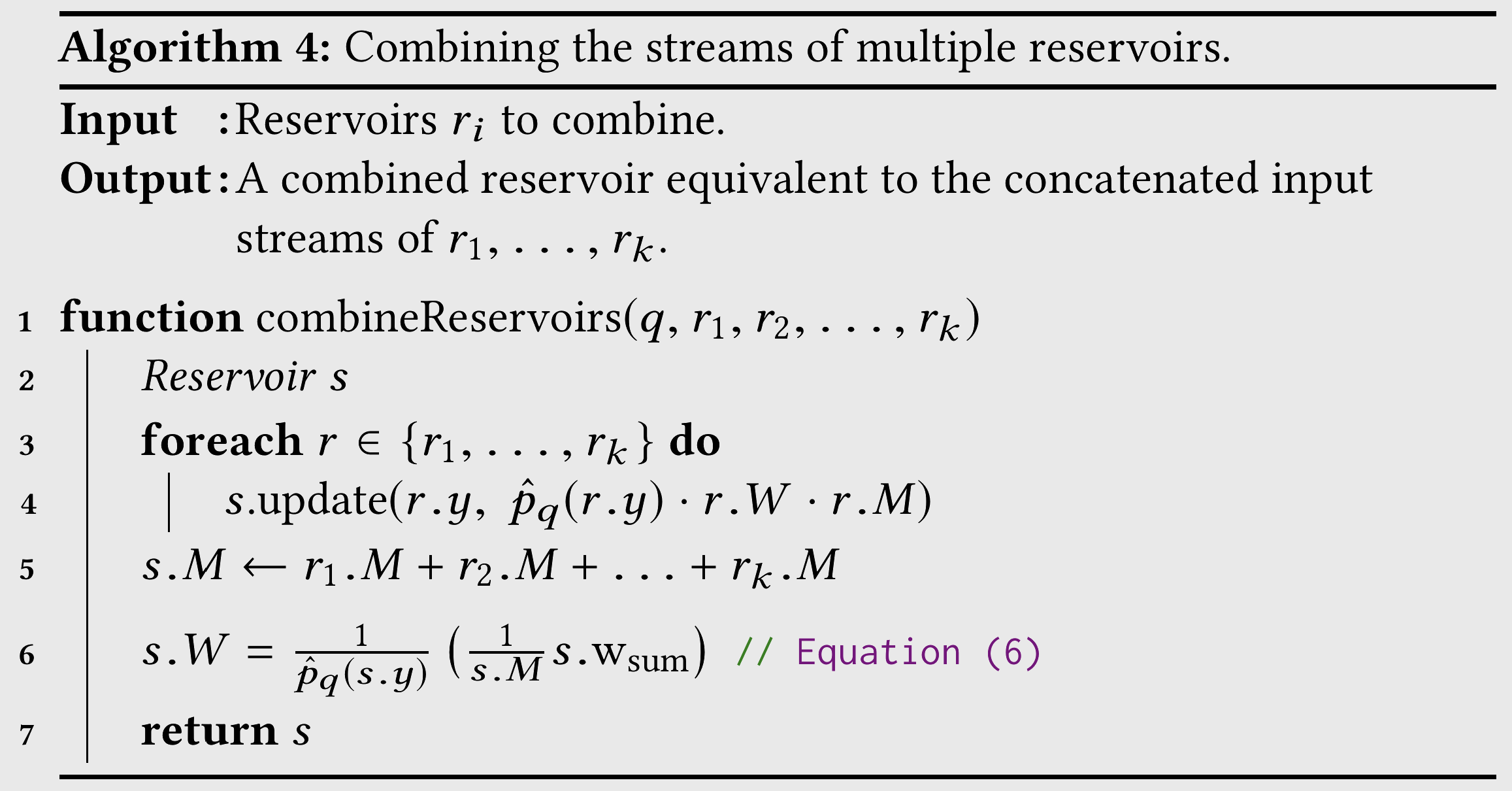
The sampling result is equivalent to directly sampling the merged sequence.

If RIS itself samples $M$ times and reuses $k$ neighbors' results, the computational complexity is $O(k+M)$, but the pixel sees $k\cdot M$ samples; if spatial reuse is repeated $n$ times, the complexity becomes $O(nk+M)$ for $k^n\cdot M$ samples.

Temporal Reuse

In animations, the reservoir from the previous frame is used to initialize the reservoir for the current frame.

This gives us a sampling method that combines WRS and RIS with temporal and spatial reuse.

Bias Analysis

Spatial reuse introduces bias into ReSTIR's sampling results. Rewriting the RIS formula: $$ \langle L\rangle_{\text{ris}}^{1,M} = \frac{f(y)}{\hat p(y)}\cdot\left(\frac{1}{M}\sum_{j=1}^M\text{w}(x_j)\right) = f(y) \cdot W(\mathbf{x},z) $$ where $$ W(\mathbf{x},z) = \frac{1}{\hat p(x_z)}\left(\frac{1}{M}\sum_{j=1}^M\text{w}(x_j)\right) $$ To align with the IS form, i.e., $\frac{f(y)}{p(y)}$, we must ensure that the expectation of $W(\mathbf{x},z)$ equals $\frac{1}{p(y)}$ to maintain unbiasedness. The following analysis shows that for a given $y$, traversing all combinations $(\mathbf{x},z)$ where $x_z = y$, the average of $W(\mathbf{x},z)$ is: $$ E_{x_z=y}[W(\mathbf{x},z)] \leq \frac{1}{p(y)} $$ Equality holds only if all PDFs of the samples $\mathbf{x}$ (note: originally we assumed $\mathbf{x} \sim p$, but after spatial reuse, we can no longer guarantee that samples from neighboring pixels come from the same distribution, so there may be many distributions) are non-zero at $y$.

Detailed Derivation

First, generalize RIS. Assume that the samples in $\mathbf x$ are drawn from different distributions, with the $i$-th sample $x_i \sim p_i$. Then: $$ p(\mathbf x) = \prod_{i=1}^M p_i(x_i) $$ Modify the resampling weights accordingly (i.e., replace $p$ with $p_i$): $$ p(z | \mathbf x) = \frac{w_z(x_z)}{\sum_iw_i(x_i)}, \text{where }w_i(x) = \frac{\hat p(x_i)}{p_i(x_i)} $$ The joint PDF of $\mathbf x, z$ is: $$ p(\mathbf x, z) = p(z|\mathbf x)\cdot p(\mathbf x) = \left[\prod_{i=1}^Mp_i(x_i)\right]\cdot \frac{w_z(x_z)}{\sum_iw_i(x_i)} $$ For a given $y$, there are many possible $\mathbf x, z$ combinations (e.g., $x_1 = y, z = 1$ or $x_M = y, z=M$). For convenience, we first define the set $Z(y)$:

$$ Z(y) = {i | 1\leq i\leq M \land p_i(y)\gt 0} $$ i.e., "the set of indices where (y) can appear in this position." Fixing index (i), the remaining (M-1) positions can be freely chosen, ensuring that (\mathbf x, z) is a combination that samples (y). Thus, (p(y)) is the sum of all (M-1) integrals: $$ p(y) = \sum_{i\in Z(y)}\int\cdots\int p(\mathbf{x}^{i\to y}, i)\text{d}x_1\cdots\text{d}x_M $$ For (W(\mathbf x, z)), the mean when the sampling result is fixed to (y) is: $$ \begin{aligned} E_{x_z=y} &= \frac{\int\cdots\int W(\mathbf{x}^{i\to y}, i)p(\mathbf{x}^{i\to y}, i)\text{d}x_1\cdots\text{d}x_M}{\int\cdots\int p(\mathbf{x}^{i\to y}, i)\text{d}x_1\cdots\text{d}x_M} \ \end{aligned} $$ A simple derivation (really simple XD, most terms cancel out) yields: $$ E_{x_z=y} = \frac{1}{p(y)} \frac{|Z(y)|}{M} \leq \frac{1}{p(y)} $$ Thus, unbiasedness is guaranteed only if (|Z(y)| = M), i.e., all PDFs are non-zero at (y). Otherwise, the result will be biased downward. Specifically, the ReSTIR algorithm discards occluded samples (effectively setting their PDF to 0), but samples occluded in neighboring pixels may not be occluded in the current pixel, leading to bias and darkening of the image.

Bias Elimination

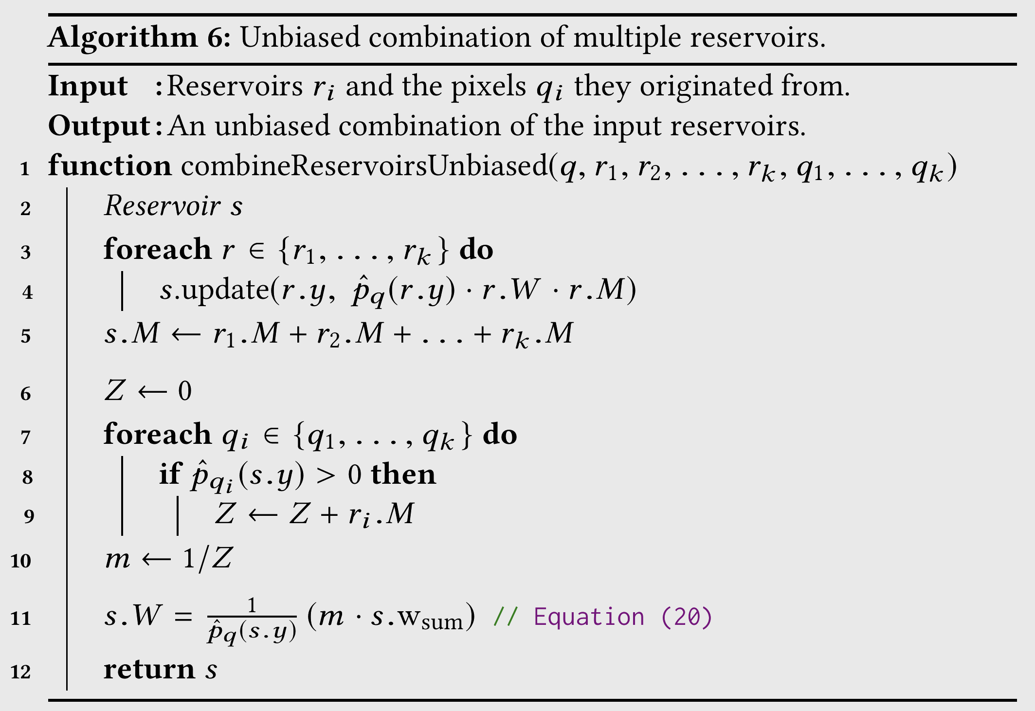
By replacing the weight $1/M$ in $W(\mathbf x, z)$ with a variable $m(x_z)$, the expectation becomes: $ E_{x_z=y} = \frac{1}{p(y)}\sum_{i\in Z(y)}m(x_i) $ Unbiasedness is then equivalent to $\sum_{i\in Z(y)}m(x_i) = 1$.

This can be achieved by simply setting $m(x_z)$ to $\frac{1}{|Z(x_z)|}$, but the result is very noisy.
A better approach is to use an MIS-like estimation for $m$, e.g.: $ m(x_z) = \frac{p_z(x_z)}{\sum_{i=1}^Mp_i(x_z)} $

In practice, the authors use $\hat p_{q_i}(x_i)$ to approximate the true PDF: as long as the true PDF is non-zero, it will also be non-zero. Below is the pseudocode for an unbiased reservoir combination algorithm using average weights (i.e., method 1 above).

Pseudocode for unbiased reservoir combination

Implementation Details

The authors implemented the ReSTIR sampler in Falcor, with the following parameters:

RIS initial sampling $M = 32$, distribution $p \propto L_e$
- If an environment map is present, 25% of the samples are importance sampled from it.
Target PDF is $\hat p \propto\ \rho \cdot L_e \cdot G$
- All BRDFs are treated as two-layer media with a Lambertian base and GGX top layer.
Selecting fixed-position neighbors can lead to artifacts, so 5 (3 for unbiased) pixels are randomly sampled from a 30px radius as neighbors.
- In the biased algorithm, neighbors with large geometric differences introduce significant bias, so the camera angle and depth are computed during sampling, and neighbors with large differences are rejected.
To achieve interactive frame rates, unbiased uses $N = 1$, biased uses $N = 4$, and offline rendering can use larger values.